NeRF 구현하기
기본적인 NeRF를 pytorch로 구현해보기
모델 구현
NeRF model
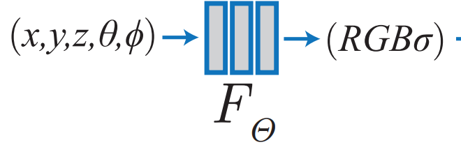
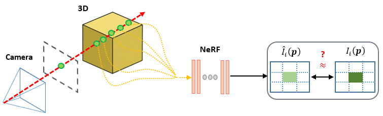
잘 아시다시피 NeRF(\(F_\theta)\) 는 3D 위치, 카메라 시점을 입력받아 RGB color, density를 출력하는 인공지능 신경망으로 구성된 함수입니다.
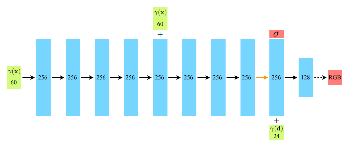
구조자체는 단순한 MLP이기 때문에 input이 새로 들어오는 부분, output 부분만 주의해서 레이어 블록을 쌓으면 됩니다.
1
2
3
4
5
6
7
8
9
10
11
12
13
14
15
16
17
18
19
20
21
22
23
24
25
26
27
28
29
30
31
32
class NerfModel(nn.Module):
    def __init__(self, embedding_dim_pos=10, embedding_dim_direction=4, hidden_dim=128):
        super(NerfModel, self).__init__()

        self.block1 = nn.Sequential(
            nn.Linear(embedding_dim_pos * 6 + 3, hidden_dim),
            nn.ReLU(),
            nn.Linear(hidden_dim, hidden_dim),
            nn.ReLU(),
            nn.Linear(hidden_dim, hidden_dim),
            nn.ReLU(),
            nn.Linear(hidden_dim, hidden_dim),
            nn.ReLU(),
        )

        self.block2 = nn.Sequential(
            nn.Linear(embedding_dim_pos * 6 + hidden_dim + 3, hidden_dim),
            nn.ReLU(),
            nn.Linear(hidden_dim, hidden_dim),
            nn.ReLU(),
            nn.Linear(hidden_dim, hidden_dim) + 1,  # 1 for dnesity
            nn.ReLU(),
        )

        self.block3 = nn.Sequential(
            nn.Linear(embedding_dim_direction * 6 + hidden_dim + 3, hidden_dim // 2),
            nn.ReLU(),
        )

        self.block4 = nn.Sequential(nn.Linear(hidden_dim // 2, 3), nn.Sigmoid())
        self.embedding_dim_pos = embedding_dim_pos
        self.embedding_dim_direction = embedding_dim_direction
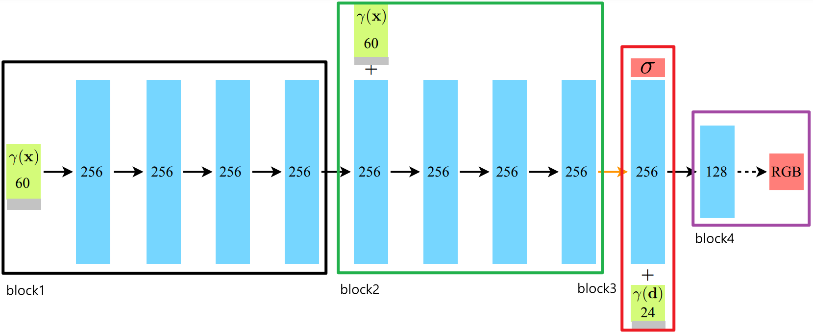
논문과 다르게 positional 임베딩 벡터의 크기가 3씩 더 큽니다.
이는 임베딩 되지 않은 원래의 값을 추가된 것인데, NeRF를 구현한 대부분의 코드가 이렇게 원래의 값을 추가하여 사용하고 있습니다.
아마, positional encoding 과정에서 원래의 값이 변형되므로 모델이 더 확실하게 위치 및 카메라 시점을 이해할 수 있도록 명시적인 값을 넣는 것 같습니다.
Positional encoding

NeRF는 positional encoding이라는 기법을 사용하는데, \(x, y, z, \phi, \theta\) 의 저차원(6차원) input으로는 high-frequency variation인 컬러 및 밀도 값을 제대로 표현할 수 없다고 합니다.
때문에 위와 같은 positional encoding 수식을 적용하여 저차원의 입력을 보다 고차원의 high frequency variation으로 만들어줍니다.
이를 코드로 구현하면 다음과 같습니다.
1
2
3
4
5
6
7
@staticmethod
def positional_encoding(x, L):
    out = [x]
    for j in range(L):
        out.append(torch.sin(2**j * x))
        out.append(torch.cos(2**j * x))
    return torch.cat(out, dim=1)
앞서 언급했듯이, 원래의 값 x가 그대로 들어가기 때문에 output의 차원은 input_dim * 2 * L + input_dim이 됩니다.
position의 경우 L = 10이므로 임베딩 후 크기는 63이며, viewing direction은 L = 4이므로 임베딩 후 크기는 27입니다.
forward
1
2
3
4
5
6
7
8
9
10
11
12
13
14
15
16
17
18
19
20
21
22
23
24
def forward(self, o, d):
    emb_x = self.positional_encoding(
        o, self.embedding_dim_pos
    )  # [batch_size, 60] : 3 * 2 * L = 10
    emb_d = self.positional_encoding(
        d, self.embedding_dim_direction
    )  # [batch_size, 24] : 3 * 2 * L = 4

    # block1
    h = self.block1(emb_x)

    # block2
    temp = torch.cat((h, emb_x), dim=1)
    h2 = self.block2(temp)
    h2, sigma = h2[:, :-1], h2[:, -1]

    # block3
    temp = torch.cat((h2, emb_d), dim=1)
    h3 = self.block3(temp)

    # block4
    color = self.block4(h3)

    return color, sigma
block2의 output 중 마지막 값이 sigma를 나타내며, block4의 output 3개가 RGB 컬러값을 나타냅니다.
렌더링 함수 구현
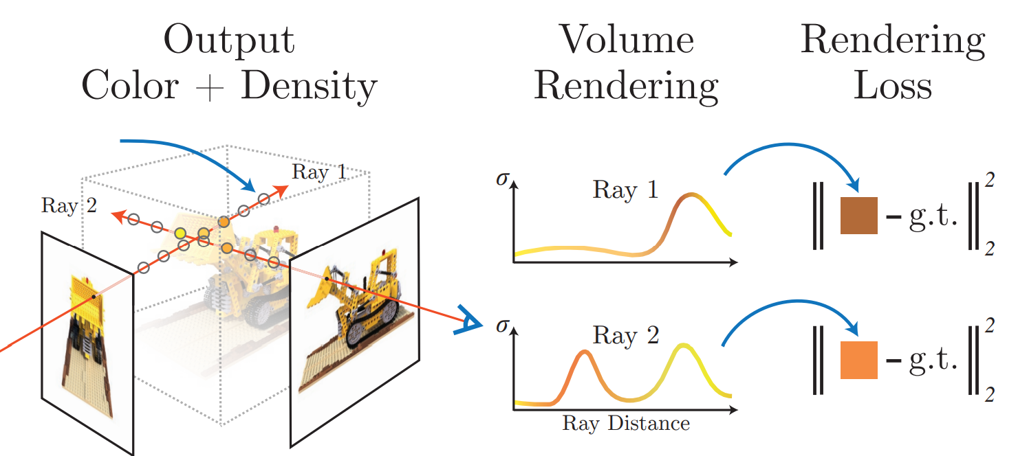
NeRF를 학습하기 위해서는, 미분 가능한 렌더링 함수를 통해 이미지를 생성하여 정답 이미지와의 차이를 계산해야 합니다.
NeRF 함수 자체만으로는 특정 지점의 컬러와 밀도값만 알 수 있기 때문에 이 값들을 합쳐 이미지를 생성하는 과정은 다음과 같습니다.
discrete point sampling

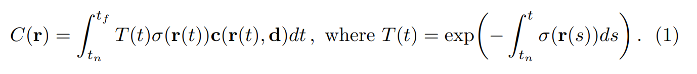
카메라 원점에서 픽셀 방향으로 ray를 쏘았을 때 해당 ray가 지나는 지점의 컬러(\(\mathbf{c}\)), 밀도(\(\sigma\))를 모두 합친 값이 해당 픽셀의 색상값이 됩니다.
하지만 위 Eq. 1 처럼 적분을 하려면 구해야 하는 point가 무한대가 되므로, 어느정도 uniform하게 샘플링하여 샘플링된 포인트의 컬러, 밀도를 합하는 식으로 픽셀의 색상을 결정합니다.
1
2
3
4
5
6
7
8
9
10
11
12
13
14
15
16
17
18
19
20
21
22
23
"""
hn: 샘플링의 시작 범위
hf: 샘플링의 끝 범위
nb_bins: 샘플링할 point 개수
"""
ticks = torch.linspace(hn, hf, nb_bins, device=device).expand(
    ray_origins.size(0), nb_bins
)

mid = (ticks[:, :-1] + ticks[:, 1:]) / 2.0
lower = torch.cat((ticks[:, :1], mid), -1)
upper = torch.cat((mid, ticks[:, -1:]), -1)

u = torch.rand(ticks.shape, device=device)
t = lower + (upper - lower) * u # 샘플링

delta = torch.cat(
    (
        t[:, 1:] - t[:, :-1],
        torch.tensor([1e10], device=device).expand(ray_origins.size(0), 1),
    ),
    -1,
)
torch.linspace()로 샘플링할 범위를 균등하게 나누고, 해당 범위 내에서 하나씩 랜덤한 포인트(\(t\))를 샘플링합니다.
delta는 이전 point와의 거리를 계산한 값입니다. 픽셀의 최종 색상을 계산할 때 사용됩니다.
get color of each sampled point
1
2
3
4
5
6
x = ray_origins.unsqueeze(1) + t.unsqueeze(2) * ray_directions.unsqueeze(1)  # [batch_size, nb_bins, 3]
ray_directions = ray_directions.expand(ray_directions.size(0), nb_bins, 3)

colors, sigma = nerf_model(x.reshape(-1, 3), ray_directions.reshape(-1, 3))
colors = colors.reshape(x.shape)
sigma = sigma.reshape(x.shape[:-1])
주어진 ray의 원점(카메라 위치)과 방향을 NeRF의 입력으로 넣어 color, sigma 값을 반환받습니다.
모델에는 flatten된 형태로 들어가야 하기 때문에 reshape(-1, 3)을 거칩니다.
volume rendering
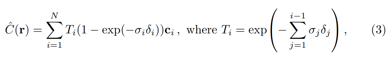
이렇게 모든 sampled point에 대한 color를 구했다면, volume rendering을 통해 해당 픽셀의 color를 계산하여 최종적으로 이미지를 렌더링 할 수 있습니다.
\(\alpha_i = 1 - exp(-\sigma_i \delta_i)\) 라고 할 경우, Eq. 3는 다음과 같습니다.
- \[\hat{C}(r) = \sum^N_{i=1}(\prod^{i-1}_{j=1}{\alpha_i}) \alpha_i \mathbf{c}_i\]
위 식을 코드로 구현하면 다음과 같습니다.
1
2
3
4
5
6
7
8
9
10
11
12
13
14
15
16
alpha = 1 - torch.exp(-sigma * delta)
weights = compute_accumulated_transmittance(alpha.unsqueeze(2)) * alpha.unsqueeze(2)
result = (weights * colors).sum(dim=1)

def compute_accumulated_transmittance(alphas):
    accumulated_transmittance = torch.cumprod(1-alphas, dim=1)
    return torch.cat(
        (
            torch.ones(
                (accumulated_transmittance.size(0), 1),
                device=accumulated_transmittance.device,
            ),
            accumulated_transmittance[:, :-1],
        ),
        dim=-1,
    )
torch.cumprod() 함수를 통해 prod 계산을 손쉽게 구현할 수 있습니다. 계산 결과를 반환할 때 \(T_1 = 1\) 이 되어야 하므로 제일 앞에 추가하여 반환합니다.
이대로 렌더링할 경우, 학습 데이터에서 배경을 제거한 경우에 배경 부분에 artifacts가 나올 수 있다고 합니다.
때문에 다음과 같이 배경부분을 흰색으로 만드는 regularization term을 사용합니다.
1
2
3
4
5
6
7
alpha = 1 - torch.exp(-sigma * delta)
weights = compute_accumulated_transmittance(alpha.unsqueeze(2)) * alpha.unsqueeze(2)
c = (weights * colors).sum(dim=1)

# Regularization Term
weight_sum = weights.sum(-1).sum(-1)
result = c + 1 - weight_sum.unsqueeze(-1)
1 - weights는 투과되지 않고 남은 빛의 비율로 해석할 수 있으므로, 남은 만큼의 값을 더해주어 해당 픽셀의 색상을 하얗게 만들어주는 역할을 합니다.
학습
1
2
3
4
5
6
7
8
9
10
11
12
13
14
15
16
17
18
19
20
21
22
23
24
25
26
27
28
29
30
def train(
    nerf_model,
    optimizer,
    scheduler,
    data_loader,
    device="cpu",
    hn=0,
    hf=1,
    nb_epochs=int(1e5),
    nb_bins=192,
):
    training_loss = []
    for _ in tqdm(range(nb_epochs)):
        for batch in data_loader:
            ray_origins = batch[:, :3].to(device)
            ray_directions = batch[:, 3:6].to(device)
            ground_truth_px = batch[:, 6:].to(device)  # [B, 3]

            pred_px = render_rays(
                nerf_model, ray_origins, ray_directions, hn, hf, nb_bins
            )

            # MSE Loss
            loss = ((ground_truth_px - pred_px) ** 2).sum()

            optimizer.zero_grad()
            loss.backward()
            optimizer.step()
            training_loss.append(loss.item())
        scheduler.step()
NeRF를 통해 렌더링 된 이미지와 GT 이미지의 차이(MSE)를 손실 함수로 사용하여 학습합니다.
코멘트
지금까지 논문을 읽어보기만 하고, 오픈소스에서 몇몇 부분을 찾아보긴 했어도, 코드를 직접 짜본적이 없었습니다.
여기저기 검색해본 결과 코드 구현에 대한 자료가 많이 존재해서 직접 따라하면서 이해해보았습니다.
논문에서는 그렇구나~하고 넘어간 부분을 생각보다 복잡한 방법으로 해야하는 경우도 있었고, 복잡한 수식이 오히려 간단한 함수로 대체되기도 해서 좀 더 새로운 관점으로 논문을 이해하게 된 것 같습니다.
참고 자료
NeRF 논문 영상 - Neural Radiance Fields | NeRF in 100 lines of PyTorch code 블로그 - NeRF : Neural Radiance Field(1)